Training a machine learning model with Zillow data for price prediction

Accurately predicting rental prices is a common regression problem with practical applications in real estate analytics. It requires handling multiple variables — location, size, amenities, property age — and building a model that generalizes well to new listings.

In this tutorial, we use Zillow listings from Cambridge, Somerville, and Boston as our machine learning training data to build a regression model for monthly rent. You’ll learn the full process: preparing and cleaning raw data, engineering features, and evaluating model performance — skills directly applicable to other machine learning prediction tasks. The Jupyter Notebook and dataset are available on GitHub or can be opened in Google Colab using the links below.

How to build a rental price prediction model

• 1) Setup
• 2) Data preparation
• 3) Data cleaning
• 4) Feature engineering
• 5) Modeling
• 6) The results
• 7) How to improve further
• 8) Scraping Zillow data for machine learning

1) Setup

Install required libraries

To start, let’s install and import all the packages we’ll need for this tutorial. From here on out, every code example will follow Jupyter Notebook formatting, meaning each snippet represents its own cell, just like in a real notebook.

# Install required packages
%pip install pandas scikit-learn matplotlib joblib scikit-optimize apify-client python-dotenv

Import libraries

# Import all the libraries we'll need for this tutorial
import json
import pandas as pd
import numpy as np
import matplotlib.pyplot as plt
from pathlib import Path

# Machine learning imports
from sklearn.model_selection import train_test_split, cross_validate, GridSearchCV
from sklearn.linear_model import LinearRegression
from sklearn.ensemble import RandomForestRegressor
from sklearn.metrics import mean_absolute_error, r2_score

print("✅ All packages installed and libraries imported successfully!")

2) Data preparation

2.1 Data loading

As mentioned earlier, in this tutorial, we’ll work with real estate data scraped from rental listings in the Greater Boston area (Boston, Cambridge, and Somerville). The data was collected from Zillow using Apify’s Zillow Search Scraper, and you can download the dataset from the GitHub link here.

With the dataset in hand, let’s load it and start exploring. Here’s what we expect to find:

• Property details (bedrooms, bathrooms, area)
• Location information (addresses, coordinates)
• Rental prices (our target variable)

data_path = Path("./data/boston-rental-properties.json")
with open(data_path) as f:
    data = json.load(f)

print(f"🏠 Successfully loaded {len(data):,} rental listings!")

2.2 Data exploration

By now, you should have your data ready and loaded into your code. Let’s start by taking a peek at its structure to get a better sense of what we’re working with. Think of this step as getting to know the ingredients before cooking a meal.

To that end, let's examine a couple of sample records to understand what information we have available:

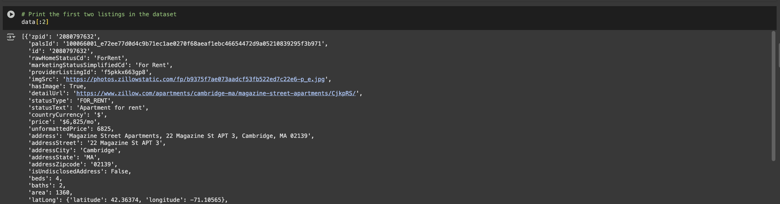
# Print the first two listings in the dataset
data[:2]

After running it, you'll get an output similar to the one below.

2.3 Creating a working dataset

The Apify Zillow Scraper gave us a well-structured, detailed dataset to work with, saving us a ton of time right from the start. But raw data alone isn’t ready to be fed into a model just yet.

We still need to pull out only the information that’s actually useful for predicting rent prices. Sticking with our kitchen analogy, this step is like picking the right ingredients from a fully stocked pantry.

What data are we looking for?

• Property characteristics: beds, baths, area (square footage)
• Location data: latitude, longitude (extracted from nested latLong field)
• Target variable: unformattedPrice (what we want to predict)
• Context: address, city, zipcode (for reference, though we won't use these in modeling)

Let's extract these fields and create a clean pandas DataFrame:

# First, let's see all available columns in our data
df_full = pd.DataFrame(data)
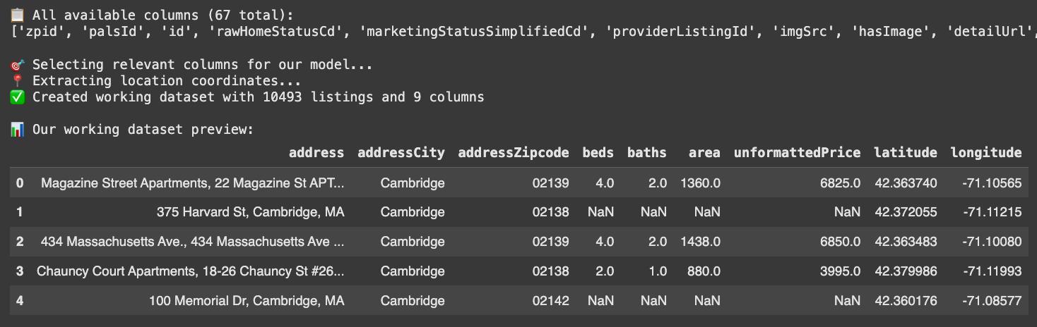
print(f"📋 All available columns ({len(df_full.columns)} total):")
print(list(df_full.columns))

# Now extract only the columns we need for rent prediction
print(f"\n🎯 Selecting relevant columns for our model...")
df_work = df_full[['address', 'addressCity', 'addressZipcode', 'beds', 'baths', 'area', 'unformattedPrice']].copy()

# Extract latitude and longitude from the nested latLong field
print(f"📍 Extracting location coordinates...")
latitude = df_full['latLong'].apply(lambda x: x.get('latitude') if isinstance(x, dict) else None)
longitude = df_full['latLong'].apply(lambda x: x.get('longitude') if isinstance(x, dict) else None)

# Add coordinates to our filtered dataframe
df_work['latitude'] = latitude
df_work['longitude'] = longitude

print(f"✅ Created working dataset with {len(df_work)} listings and {len(df_work.columns)} columns")
print(f"\n📊 Our working dataset preview:")
df_work.head()

The data is looking much more digestible, but we are not done. We selected our features, but now we're facing another issue: some rows are missing key data points that we will need to train our model. Let’s handle them in the next section.

3) Data cleaning

You might’ve noticed some pesky NaN values when we visualized the dataset earlier. Real-world data is rarely perfect. And just like you wouldn’t start cooking without washing your veggies (at least, I hope you wouldn’t), we shouldn’t train a model without giving our data a good clean first.

Why cleaning matters?

• Missing values can crash our model or give weird predictions
• Outliers (like a 50-bedroom apartment) can throw off our model's learning
• Impossible values (negative square footage) indicate data errors

How can we clean this dataset?

1. Remove missing values: Drop listings missing critical information
2. Remove outliers: Use statistical methods to identify and remove extreme values
3. Validate data: Ensure all values make sense (positive areas, reasonable prices)

3.1 Handling missing values

Let's start by checking for missing data and dropping some “faulty” rows while we are at it:

# First, let's see how much missing data we have
missing_data = df_work.isnull().sum()
for column, missing_count in missing_data.items():
    if missing_count > 0:
        percentage = (missing_count / len(df_work)) * 100
        print(f"{column}: {missing_count} missing ({percentage:.1f}%)")

print(f"\n📊 Total listings before cleaning: {len(df_work):,}")

# Remove listings with missing critical data
listings_before_drop = len(df_work)
df_filtered = df_work.dropna()
listings_after_drop = len(df_filtered)

removed_count = listings_before_drop - listings_after_drop
removal_percentage = (removed_count / listings_before_drop) * 100

print(f"🗑️  Removed {removed_count:,} listings due to missing data ({removal_percentage:.1f}%)")
print(f"✅ Clean dataset now has {listings_after_drop:,} listings")

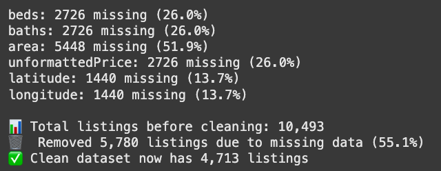
Over half our rows were missing at least one key feature, so we ended up tossing about 55% of the dataset. Sounds bad, but bad data hurts a model more than less data; quality wins over quantity.

In real projects, you’d usually fill in those gaps (imputation, predictions, extra data sources), but we’ll skip that here to keep things simple. Just keep in mind that: handling missing data well can save more samples and boost model performance.

3.2 Outlier detection and removal

The missing data rows are gone, but that’s not the only thing that can affect our dataset quality. Outliers are a common and dangerous occurrence in any data, especially in user-generated data without any quality control, like Zillow’s, which might cause users to input wrong or unrealistic values.

What are outliers?

In short, outliers are data points that are extremely different from the typical values. For example:

• A 20-bedroom apartment (might be a data entry error)
• A $50,000/month studio (probably a typo)
• A 10,000 square foot "apartment" (might be a commercial space)

How to deal with outliers?

While there are many ways of handling outliers, and the method choice depends on the characteristics of the data you are working with, for our use case, we'll go with the IQR (Interquartile Range) method to detect outliers. This is how the IQR works:

• Calculate Q1 (25th percentile) and Q3 (75th percentile)
• Anything below Q1 - 1.5×IQR or above Q3 + 1.5×IQR is considered an outlier

# Remove outliers using the IQR method
def remove_outliers_iqr(df, columns):
    """
    Remove outliers using the IQR (Interquartile Range) method.
    """

    df_clean = df.copy()

    print(f"\n🔧 Applying outlier removal:")

    for column in columns:
        # Calculate quartiles and IQR
        Q1 = df_clean[column].quantile(0.25)
        Q3 = df_clean[column].quantile(0.75)
        IQR = Q3 - Q1

        # Define outlier bounds
        lower_bound = Q1 - 1.5 * IQR
        upper_bound = Q3 + 1.5 * IQR

        # Remove outliers
        before_count = len(df_clean)
        df_clean = df_clean[(df_clean[column] >= lower_bound) & (df_clean[column] <= upper_bound)]
        after_count = len(df_clean)

        removed = before_count - after_count
        print(f"   • {column}: removed {removed} outliers (bounds: {lower_bound:.0f} - {upper_bound:.0f})")

    # Additional business logic filter
    before_area_filter = len(df_clean)
    df_clean = df_clean[df_clean['area'] < 9000]  # Remove unreasonably large areas
    area_removed = before_area_filter - len(df_clean)
    if area_removed > 0:
        print(f"   • Additional filter: removed {area_removed} listings with area > 9000 sq ft")

    return df_clean

# Apply outlier removal
numeric_cols = ['beds', 'baths', 'area', 'unformattedPrice']
df_clean = remove_outliers_iqr(df_filtered, numeric_cols)

# Summary of cleaning results
initial_count = len(df_filtered)
final_count = len(df_clean)
total_removed = initial_count - final_count
removal_rate = (total_removed / initial_count) * 100

print(f"\n📊 CLEANING SUMMARY:")
print(f"   • Started with: {initial_count:,} listings")
print(f"   • Removed: {total_removed:,} outliers ({removal_rate:.1f}%)")
print(f"   • Final dataset: {final_count:,} clean listings")
print(f"   • Data retention rate: {(final_count/initial_count)*100:.1f}%")

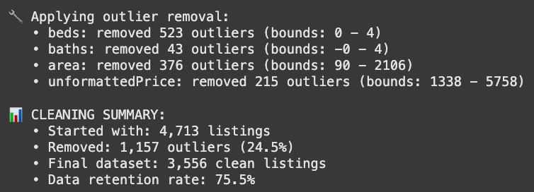
Outliers removed, and we’re left with 3,556 clean, complete listings out of the 10k we started with. Not bad, especially since we didn’t have to use any fancy data imputation tricks to get here.

4) Feature engineering

Now that our data is clean, it's time to prepare it for machine learning.

Starting by adding new features to our dataset through a process called Feature Engineering. This means creating new features from existing ones, basically giving our model extra “clues” to help it make better predictions.

# Step 1: Select our base features for modeling
base_features = ['beds', 'baths', 'area', 'latitude', 'longitude']

# Step 2: Engineer additional features that might be helpful
df_clean['totalRooms'] = df_clean['beds'] + df_clean['baths']
print("✅ Created 'totalRooms' = beds + baths")

# Final feature list
final_features = base_features + ['totalRooms']
print(f"\n📊 Final feature set ({len(final_features)} features):")
print(final_features)

# Prepare our feature matrix (X) and target variable (y)
X = df_clean[final_features]
y = df_clean['unformattedPrice']

print(f"\n📈 Dataset Summary:")
print(f"   • Features (X): {X.shape[0]:,} samples × {X.shape[1]} features")
print(f"   • Target (y): {len(y):,} rent prices")
print(f"   • Target range: ${y.min():,.0f} - ${y.max():,.0f}")
print(f"   • Average rent: ${y.mean():,.0f}")

# Quick peek at our engineered dataset
print(f"\n👀 Feature Preview:")
X.head()

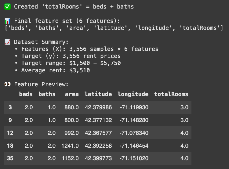
And just like that, our newly engineered feature is part of the dataset. It might seem trivial now, but later you’ll see that even a single, simple but meaningful feature can make a noticeable difference in our model’s performance.

5) Modeling

5.1 Train/Test split + baseline model

Now that all features are in place, it’s time for one of the most important steps in building a model: splitting the data.

Train/Test Split means dividing our data into two parts:

• Training set (80%): The data our model learns from
• Test set (20%): The data we keep hidden until the end to see how well the model really performs on something new

This split is essential to prevent overfitting. We want our model to handle fresh, never-before-seen rental listings, not just ace the “exam” by memorizing the practice questions.

# Create train/test split to evaluate our model properly
X_train, X_test, y_train, y_test = train_test_split(
    X, y, 
    test_size=0.2,      # 20% for testing, 80% for training
    random_state=42     # For reproducible results
)

print(f"📊 Split summary:")
print(f"   • Training set: {len(X_train):,} listings ({len(X_train)/len(X)*100:.0f}%)")
print(f"   • Test set: {len(X_test):,} listings ({len(X_test)/len(X)*100:.0f}%)")
print(f"   • Average rent in training: ${y_train.mean():,.0f}")
print(f"   • Average rent in test: ${y_test.mean():,.0f}")

# Quick baseline: Let's see how our first simple linear regression model performs
baseline_model = LinearRegression()
baseline_model.fit(X_train, y_train)

# Make predictions and evaluate
y_pred_baseline = baseline_model.predict(X_test)
baseline_mae = mean_absolute_error(y_test, y_pred_baseline)
baseline_r2 = r2_score(y_test, y_pred_baseline)

print(f"\n📈 Baseline Performance:")
print(f"   • MAE (Mean Absolute Error): ${baseline_mae:,.0f}")
print(f"   • R² (R-squared): {baseline_r2:.3f}")
print(f"\n💡 What this means:")
print(f"   • On average, our predictions are off by ${baseline_mae:,.0f}")
print(f"   • Our model explains {baseline_r2:.1%} of rent price variation")
print("   • Room for improvement - let\'s try more advanced models!")

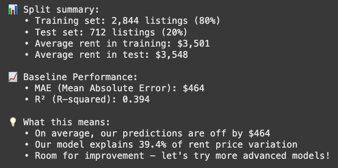
We kicked things off with a simple Linear Regression model, but with an R² of just 39.4% for rent price variation, it’s not exactly impressive. Next, we’ll try out a different model to see if we can do better.

5.2 Model comparison - Finding the best algorithm

Our baseline linear regression gave us a starting point, but its performance is far from ideal. When a model scores this low, it often means the underlying data patterns are more complex than the model can capture.

In cases like this, a good next step is to try different algorithms, compare them using cross-validation, and pick a “champion” model, one that gives us the strongest baseline for further tuning and optimization later on.

Why try different models?

• Linear Regression assumes a straight-line relationship between features and price
• Random Forest can capture complex, non-linear patterns (like "location matters more for expensive areas")
• Real estate prices often have complex relationships that linear models miss

How to compare models

• Use cross-validation (test on 5 different data splits) for reliable performance estimates
• Compare MAE (average prediction error in dollars) and R² (explained variance)
• Watch for overfitting because we want a model that generalizes, not one that just memorizes the training data

Let's see which algorithm works best for our data.

# Define our models to compare
models = {
    'Linear Regression': LinearRegression(),
    'Random Forest': RandomForestRegressor(
        n_estimators=100,       # Number of trees
        max_depth=10,           # Maximum tree depth  
        min_samples_split=5,    # Minimum samples to split
        random_state=42,        # For reproducible results
        n_jobs=-1               # Use all CPU cores
    )
}

def evaluate_models_with_cv(models, X, y, cv_folds=5):
    """
    Evaluate multiple models using cross-validation.

    Returns detailed performance metrics including overfitting analysis.
    """
    results = {}

    for name, model in models.items():
        print(f"🎯 Evaluating {name}...")

        # Perform cross-validation with multiple metrics
        cv_results = cross_validate(
            model, X, y, 
            cv=cv_folds,
            scoring=['neg_mean_absolute_error', 'r2'],
            return_train_score=True
        )

        # Calculate test metrics
        test_mae = -cv_results['test_neg_mean_absolute_error'].mean()
        test_mae_std = cv_results['test_neg_mean_absolute_error'].std()
        test_r2 = cv_results['test_r2'].mean()
        test_r2_std = cv_results['test_r2'].std()

        # Calculate train metrics (to check overfitting)
        train_mae = -cv_results['train_neg_mean_absolute_error'].mean()
        train_r2 = cv_results['train_r2'].mean()

        # Overfitting indicators
        overfit_mae = train_mae - test_mae  # Positive = overfitting
        overfit_r2 = train_r2 - test_r2    # Positive = overfitting

        # Store results
        results[name] = {
            'test_mae': test_mae,
            'test_mae_std': test_mae_std,
            'test_r2': test_r2,
            'test_r2_std': test_r2_std,
            'overfit_mae': overfit_mae,
            'overfit_r2': overfit_r2
        }

        # Print detailed results
        print(f"   📊 Test MAE: ${test_mae:,.0f} (±${test_mae_std:,.0f})")
        print(f"   📊 Test R²: {test_r2:.3f} (±{test_r2_std:.3f})\n")

    return results

# Run the model comparison
model_results = evaluate_models_with_cv(models, X_train, y_train)

# Create and display comparison summary
comparison_df = pd.DataFrame(model_results).T
comparison_df = comparison_df.round(2)

# Display the key metrics
print(comparison_df[['test_mae', 'test_r2', 'overfit_mae']])

# Identify the best model
best_model_name = comparison_df['test_r2'].idxmax()
best_r2 = comparison_df.loc[best_model_name, 'test_r2']
best_mae = comparison_df.loc[best_model_name, 'test_mae']

print(f"\n🥇 Best model: {best_model_name}")
print(f"   • R²: {best_r2:.3f} (explains {best_r2:.1%} of price variation)")
print(f"   • MAE: ${best_mae:,.0f} (average prediction error)")

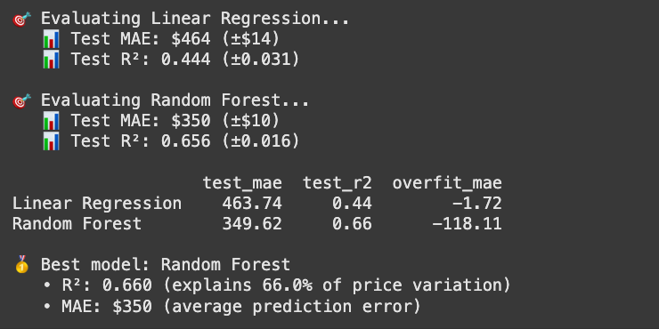
From our comparison, the Random Forest model clearly outperformed Linear Regression on this dataset. For simplicity, we only compared it against one other model here, but the same approach can be used to test multiple algorithms against each other and choose the best baseline for your data.

5.3 Hyperparameter tuning

We’ve identified our best-performing algorithm: Random Forest. Now it’s time to fine-tune it and squeeze out as much performance as we can.

Hyperparameter tuning isn’t strictly necessary, especially when our baseline is already doing reasonably well without it, but it’s often worth the effort.

Even if the gains aren’t as dramatic as adding more data, engineering better features, or switching to a more suitable algorithm, tuning can still give your model a valuable performance boost.

Why bother tuning hyperparameters?

• Squeeze out extra accuracy and stability from the model
• Find the sweet spot between underfitting and overfitting
• Adapt the model to the unique quirks of our dataset
• Avoid wasting capacity. There’s no point in having 500 trees if 200 get you the same results

# Define parameter grid to search
param_grid = {
    'n_estimators': [100, 200, 300],
    'max_depth': [10, 15, 20, None],
    'min_samples_split': [2, 5, 10],
    'min_samples_leaf': [1, 2, 4]
}

# Establish a proper CV baseline for the true default RF
rf_default = RandomForestRegressor(random_state=42, n_jobs=-1)
cv_baseline = cross_validate(
    rf_default, X_train, y_train,
    cv=5,
    scoring=['neg_mean_absolute_error', 'r2'],
    return_train_score=False
)
baseline_cv_mae = -cv_baseline['test_neg_mean_absolute_error'].mean()
baseline_cv_r2 = cv_baseline['test_r2'].mean()

# Set up and run grid search - OPTIMIZING FOR MAE
print("🚀 Running GridSearchCV...")
grid_search = GridSearchCV(
    RandomForestRegressor(random_state=42, n_jobs=-1),
    param_grid,
    scoring={'neg_mae': 'neg_mean_absolute_error', 'r2': 'r2'},
    refit='r2',
    cv=5,
    n_jobs=-1,
    verbose=1
)

grid_search.fit(X_train, y_train)

# Get best model and evaluate
best_rf = grid_search.best_estimator_

# Extract CV metrics for the best params
best_idx = grid_search.best_index_
cv_results = grid_search.cv_results_
tuned_cv_mae = -cv_results['mean_test_neg_mae'][best_idx]
tuned_cv_r2 = cv_results['mean_test_r2'][best_idx]

# Evaluate on the held-out test set once (final check)
y_pred_default = rf_default.fit(X_train, y_train).predict(X_test)
y_pred_tuned = best_rf.predict(X_test)

print("\n📊 CROSS-VALIDATION (5-fold) COMPARISON")
print(f"   Default RF (true defaults)  → CV MAE: ${baseline_cv_mae:,.0f} | CV R²: {baseline_cv_r2:.3f}")
print(f"   Tuned RF (best params)      → CV MAE: ${tuned_cv_mae:,.0f} | CV R²: {tuned_cv_r2:.3f}")

print("\n📊 TEST SET (held-out) COMPARISON")
print(f"   Default RF MAE: ${mean_absolute_error(y_test, y_pred_default):,.0f} | R²: {r2_score(y_test, y_pred_default):.3f}")
print(f"   Tuned RF MAE:   ${mean_absolute_error(y_test, y_pred_tuned):,.0f} | R²: {r2_score(y_test, y_pred_tuned):.3f}")
print(f"\n   Best params: {grid_search.best_params_}")

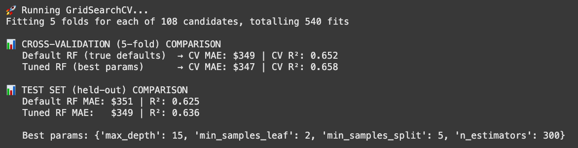
In this case, we’re focusing on optimizing the model to reduce our MAE. For rental price prediction, a lower MAE means narrowing the average gap between the model’s predictions and the actual prices. We improved from a MAE of $351 to $349—a change that might look negligible at first glance.

But small gains still count, especially when they make the model more stable and reliable on unseen data. In real-world ML applications, even a modest 1% improvement can be worth its weight in gold.

Why didn’t tuning give us bigger gains?

Hyperparameter tuning is valuable, but it’s not a magic switch that instantly doubles performance. Here’s why:

• Diminishing returns – The biggest jumps usually come from better features or cleaner data, not just parameter tweaks.
• Strong baseline – If your model is already performing well, there’s less room for dramatic improvement.
• Trade-offs matter – Some settings boost accuracy but slow down predictions, which might not be worth it in production.
• Random Forest is forgiving – Unlike algorithms such as gradient boosting, Random Forest isn’t overly sensitive to small parameter changes, so improvements tend to be incremental.

5.4 Feature importance

Now that our Random Forest is tuned, let’s peek under the hood to see what’s actually driving its predictions. A feature importance plot shows each feature’s relative contribution to the model’s output.

# Feature importance
feature_importance = pd.DataFrame({
    'Feature': X_train.columns,
    'Importance': best_rf.feature_importances_
}).sort_values('Importance', ascending=False)

# Visualize as a bar chart
import matplotlib.pyplot as plt
from matplotlib.ticker import PercentFormatter

top_n = min(20, len(feature_importance))
fi_top = feature_importance.head(top_n)

fig, ax = plt.subplots(figsize=(10, 6))
ax.barh(fi_top['Feature'], fi_top['Importance'], color='forestgreen', alpha=0.85)
ax.invert_yaxis()  # Highest importance at the top
ax.set_xlabel('Relative Importance')
ax.set_title('Random Forest Feature Importance')
ax.xaxis.set_major_formatter(PercentFormatter(1.0))  # RF importances sum to 1

# Annotate each bar
for i, v in enumerate(fi_top['Importance'].values):
    ax.text(v + 0.005, i, f"{v:.3f}", va='center')

plt.tight_layout()
plt.show()

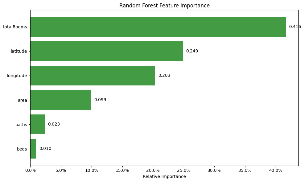
Surprise, surprise, the feature we engineered earlier ended up topping the importance chart. But at first glance, this might feel contradictory. The least important features are the number of baths and beds individually, yet the most important one – totalRooms – is just the sum of those two “least important” features. Why?

In short, Random Forest cares about how features interact with the target, not just their standalone power. Beds and baths on their own might not have strong, consistent relationships with rent, maybe because some listings have huge bedrooms but low rent, or small units with luxury finishes. But when you combine them into totalRooms, we capture a more robust signal: overall space. This aggregated feature smooths out the noise and becomes a more reliable predictor.

5.5 Sanity-checking the model

Before we put too much trust in a model, it’s worth taking a quick peek “under the hood.” Plotting a few diagnostics can reveal where the model performs well, where it struggles, and whether its errors are balanced.

So, why bother?

• Spot bias – If the model keeps overpricing cheaper rentals or underpricing expensive ones, we might be missing key features.
• Catch error trends – If errors grow with price, we may need extra information (like location perks) or data transformations.
• Compare models – The model with predictions hugging the diagonal and residuals clustered around zero usually comes out on top.

# Set up the visualization
fig, axes = plt.subplots(2, 2, figsize=(16, 12))
fig.suptitle('Linear Regression vs Tuned Random Forest', 
             fontsize=16, fontweight='bold')

# Prepare data for both models
lr_model = LinearRegression()
lr_model.fit(X_train, y_train)
y_pred_lr = lr_model.predict(X_test)
y_pred_rf = best_rf.predict(X_test)

# Calculate metrics
lr_mae = mean_absolute_error(y_test, y_pred_lr)
lr_r2 = r2_score(y_test, y_pred_lr)
rf_mae = mean_absolute_error(y_test, y_pred_rf)
rf_r2 = r2_score(y_test, y_pred_rf)

# 1. Random Forest: Predicted vs Actual
axes[0, 0].scatter(y_test, y_pred_rf, alpha=0.6, color='forestgreen', s=30)
axes[0, 0].plot([y_test.min(), y_test.max()], [y_test.min(), y_test.max()], 
               'r--', lw=2, label='Perfect Prediction')
axes[0, 0].set_xlabel("Actual Rent ($)", fontsize=12)
axes[0, 0].set_ylabel("Predicted Rent ($)", fontsize=12)
axes[0, 0].set_title(f"Tuned Random Forest\nMAE: ${rf_mae:,.0f} | R²: {rf_r2:.3f}", 
                    fontsize=13, fontweight='bold')
axes[0, 0].grid(True, alpha=0.3)
axes[0, 0].legend()

# 2. Random Forest: Residuals plot
residuals_rf = y_test - y_pred_rf
axes[1, 0].scatter(y_pred_rf, residuals_rf, alpha=0.6, color='forestgreen', s=30)
axes[1, 0].axhline(y=0, color='r', linestyle='--', lw=2)
axes[1, 0].set_xlabel("Predicted Rent ($)", fontsize=12)
axes[1, 0].set_ylabel("Residuals ($)", fontsize=12)
axes[1, 0].set_title("Random Forest Residuals", 
                    fontsize=13, fontweight='bold')
axes[1, 0].grid(True, alpha=0.3)

# 3. Linear Regression: Predicted vs Actual  
axes[0, 1].scatter(y_test, y_pred_lr, alpha=0.6, color='steelblue', s=30)
axes[0, 1].plot([y_test.min(), y_test.max()], [y_test.min(), y_test.max()], 
               'r--', lw=2, label='Perfect Prediction')
axes[0, 1].set_xlabel("Actual Rent ($)", fontsize=12)
axes[0, 1].set_ylabel("Predicted Rent ($)", fontsize=12)
axes[0, 1].set_title(f"Linear Regression\nMAE: ${lr_mae:,.0f} | R²: {lr_r2:.3f}", 
                    fontsize=13, fontweight='bold')
axes[0, 1].grid(True, alpha=0.3)
axes[0, 1].legend()

# 4. Linear Regression: Residuals plot
residuals_lr = y_test - y_pred_lr
axes[1, 1].scatter(y_pred_lr, residuals_lr, alpha=0.6, color='steelblue', s=30)
axes[1, 1].axhline(y=0, color='r', linestyle='--', lw=2)
axes[1, 1].set_xlabel("Predicted Rent ($)", fontsize=12)
axes[1, 1].set_ylabel("Residuals ($)", fontsize=12)
axes[1, 1].set_title("Linear Regression Residuals", 
                    fontsize=13, fontweight='bold')
axes[1, 1].grid(True, alpha=0.3)

plt.tight_layout()
plt.subplots_adjust(top=0.90)
plt.show()

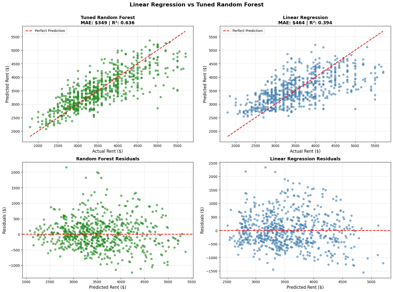
What the Random Forest plots tell us (and how it compares with Linear Regression)

• Predicted vs. Actual (top left) – The green points hug the diagonal much more tightly than the blue points from Linear Regression, showing what a “better fit” looks like in practice. Most mid-range prices line up well, though the model still underestimates some of the highest rents and slightly overestimates a few at the lower end. This suggests there are factors, like luxury amenities or very specific neighborhood effects, that our current features don’t fully capture.
• Residuals vs. Predicted (bottom left) – Residuals stay centered around zero with no strong patterns, which is exactly what we want. Compared to Linear Regression’s residuals, the spread here is tighter and more balanced, especially in the $3,000–$4,000 range, where our data is densest. At the extremes, errors widen a bit, again hinting at missing features for those outlier cases.

6) The results

6.1 Model performance

In this guide, we trained a rental price prediction model using structured Zillow data collected with an Apify scraper. Our resulting model achieved an average error rate of about $349 and the ability to explain roughly 64% of price variation. Not bad at all, given our limited dataset and just a touch of feature engineering.

6.2 Key takeaways

This tutorial demonstrated how effective it is to start with well-structured data, and how nice it is not to have to waste our time wrestling with web scraping. Apify Store has over 6,000 ready-made scrapers just like the one we used here; that's plenty of raw material for your next ML project.

7) How to improve further

Our final plots showed the model holding up pretty well, but they also hinted at where it struggles, and how we could improve it. If you’re up for a challenge, here are a few next steps:

a. Gather more data

A bigger, more diverse dataset helps the model generalize better. Try adding listings from Apartments.com or even Airbnb, depending on your use case.

b. Enrich what you have

We dropped over half our original 10,000 listings due to missing key info. Filling those gaps could dramatically increase training data. You could:

• Use geolocation APIs for location-based attributes.
• Pull extra details with the Zillow Detail Scraper.

c. Double down on feature engineering

We only added one new feature here, but you can create many more. For example, distance to major points of interest, like universities, parks, or transit hubs, often correlates strongly with rent and could give the model a serious boost.

8) Scraping Zillow data for machine learning

In this article, we’ve been working with a Zillow listings dataset pulled using Apify’s Zillow Search Scraper. But let’s be honest, you probably don’t care that much about predicting rent prices in the Greater Boston area. You’d rather do it for your own city, right?

In this final section, I’ll show you exactly how I gathered the Greater Boston dataset so you can grab data for any location you want to build your own prediction model.

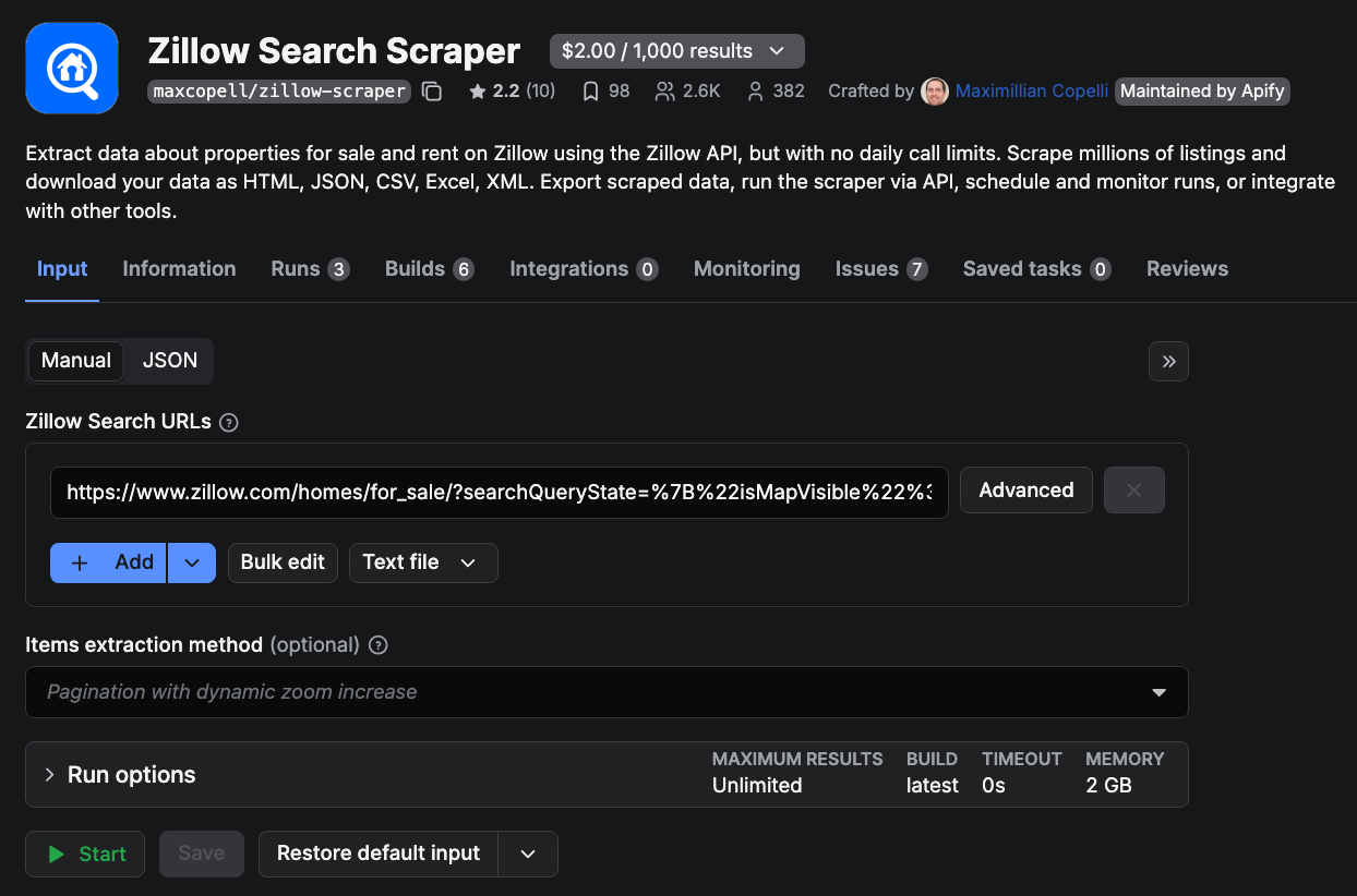
8.1 Apify scraper setup

You can access the scraper we’re using here.

If you don’t have an Apify account yet, you can create one for free.

Once you’re logged in, you’ll see the scraper’s UI, similar to the one below. The inputs are simple; you just need a Zillow search URL with the filters and settings you want. From there, click Start to begin scraping, and in just a few minutes, your dataset will be ready to export.

Below, I’ll also show you how to use the Apify CLI to call this scraper programmatically and pull the data directly into your code.

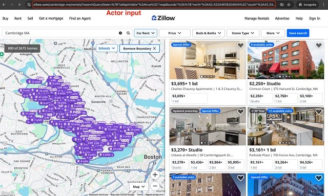
Here’s where you’ll grab the Zillow URL to give the scraper as input. In the example below, we’re looking at Zillow search for rentals in Cambridge, MA.

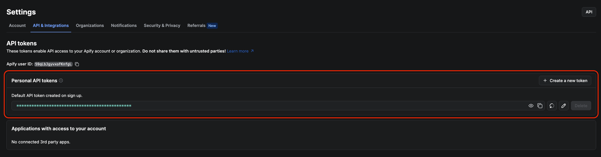
Now that your input URL is ready and your Apify account is set up, the next step is to grab your APIFY_API_TOKEN and save it in a .env file for the upcoming code snippets to work.

To find your API token, head to your Apify Console, go to Settings → API & Integrations, and copy your personal token.

8.2 Using the Apify CLI

With your APIFY_API_TOKEN safely stored in a .env file, you’re ready to run the scraper using the Apify CLI. Just swap out the dummy URL in the code below for your own.

from apify_client import ApifyClient
from dotenv import load_dotenv
import os, json

load_dotenv()
client = ApifyClient(os.getenv("APIFY_API_TOKEN"))

run_input = {
    "searchUrls": [
        {
            # Paste any Zillow search URL you’d run in the browser
            "url": "https://www.zillow.com/boston-ma/rentals/?searchQueryState=..."
        }
    ]
}

run = client.actor("maxcopell/zillow-scraper").call(run_input=run_input)
items = list(client.dataset(run["defaultDatasetId"]).iterate_items())

Path("data").mkdir(exist_ok=True)
with open("data/zillow_rentals.json", "w") as f:
    json.dump(items, f)

data = items
print(f"🏠 Scraped {len(data):,} rental listings!")

You now have a dataset for your city, similar to the one we used in this tutorial.

Use Apify for machine learning training data

Zillow Scraper isn't the only tool on Apify Store that collects web data for training machine learning models. There are over 6,000 tools built to extract data from specific websites at scale. You can use that data to give ML applications the information they need to learn and perform the tasks you're training them for.