Sentiment analysis in Python (Complete guide for 2024)

Natural Language Processing (NLP) has countless applications, and sentiment analysis is one of the most important. In this article, we’ll explore sentiment analysis in detail, from the basics and model training to tools like VADER and WordCloud. Theoretical concepts are paired with Python implementations, so I recommend opening your preferred IDE—whether VS Code, PyCharm, or Jupyter notebooks—and practicing as you go.

What is sentiment analysis?

Sentiment analysis in NLP identifies the emotional tone of text. It can classify text as positive, negative, or neutral, or use more complex categories. For instance, “the weather is pleasant” or “it is a happy morning for the English bowlers” are positive, while “the decrease in GDP growth is alarming” is negative. Neutral examples include statements like “This meeting is scheduled at 4 PM.”

A more advanced form, multi-sentiment analysis, is seen in tools like Grammarly, which uses multiple emojis to convey tone.

Prerequisites for sentiment analysis in Python

For sentiment analysis or any NLP task in Python, you don’t need an arsenal of libraries. All you need to have is Python (3+) and some relevant libraries like NLTK and WordCloud.

It's preferable to set up an environment while working in Python. This makes it much easier to maintain different environments for different types of projects without any conflicts.

Setting up the environment

You can set up the environment using Anaconda (CLI or GUI), PyCharm, or VS Code. All offer a graphical user interface for environment setup and library installation (I find Anaconda the easiest). If you prefer the command line, you can use Python's built-in tool, venv, with this command:

python -m venv nlp_env

So far, we've created the environment (in this case, nlp_env). Since you’ll likely have multiple environments, you need to activate the one you want to use with this command:

source nlp_env/bin/activate

Once activated, you can install the necessary libraries. For this tutorial, I'll install the following:

pip install numpy pandas matplotlib nltk torch

As you can see, it's quite simple. We can also check all the libraries installed within an environment by pip list.

Now our environment is set up and required libraries are also installed. So let's begin.

1. Data collection for sentiment analysis

Before choosing a source and collecting data for sentiment analysis, consider these factors:

• Volume of data needed
• Variety of sources
• Available computational power
• Cost vs. project budget

Public datasets

The easiest option is public datasets, with platforms like Kaggle, the UCI repository, and Hugging Face providing a wealth of resources.

One repository that's particularly worth exploring is the Hugging Face datasets, which are contributed by the public and constantly growing.

For benchmarking, you may also want to check out NeurIPS’s Datasets and Benchmarks Track.

However, public datasets have their limitations. Some of the challenges I faced were that the data was:

• Out of date
• Didn't align with my project goal
• Focused on specific languages and regions

Web scraping

In my experience, many ML/NLP engineers rely heavily on public datasets without exploring the potential of web scraping. This method can fetch tailored, up-to-date data with minimal effort.

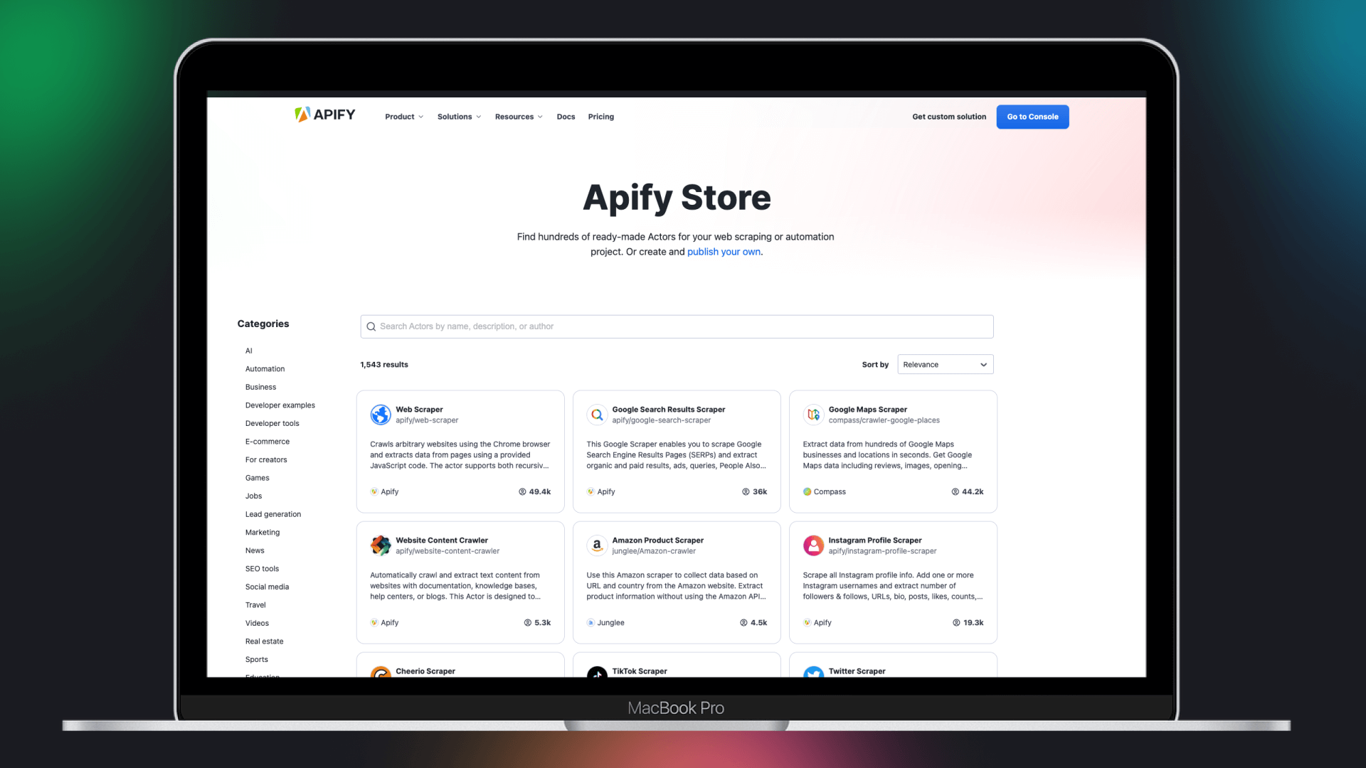
Web scraping is the automated extraction of data from websites. With the vast amount of information available online, it’s a highly valuable method. When I first learned about it in 2017, I was impressed by its potential. Now, with tools like Apify and its automated Actors, web scraping is even more practical.

If you’re new to web scraping, I recommend starting with a beginner’s guide to understand what it is and which tool fits your needs.

Twitter data

For this tutorial, we'll use Tweets as the data source. I find Twitter (now X) an ideal platform for several reasons:

• Novelty: X often covers stories that traditional media either misses or avoids.
• Speed: News spreads rapidly on this platform.
• Authenticity: Despite bots and trolls, X can offer verifiable, high-quality information when used carefully.
• Power of words: With its character limit (currently 280), X promotes concise, information-dense content, making it easier to process than longer posts on platforms like Facebook.

For Twitter, I'll use Apify's Twitter URL Scraper.

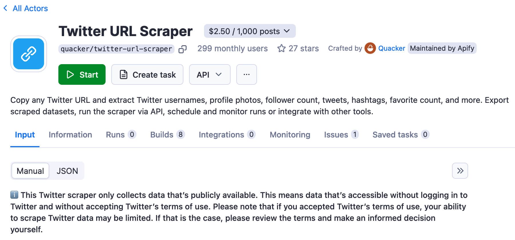
We can specify the Twitter profile (or profiles) and it will scrape the publicly available tweets.

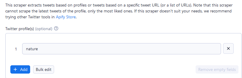
I ran the scraper several times to gather around 1,700 Tweets—not a huge amount, but enough for my purposes. I saved them as a CSV (other formats work too) to make concatenation easier.

Loading data

Now that we've scraped the data, we need to load it. Loading data in Python is incredibly simple if you use Pandas. For example, to read a CSV file:

import pandas as pd

tweets_data = pd.read_csv("SavedTweets.csv")

You can also use read_json() for JSON files. I prefer importing files into a DataFrame since it offers easy tabular visualization, handy methods, and SQL-like joins.

2. Text preprocessing

Before using data in a model, it must be preprocessed before entering the training pipeline, especially with text. Challenges like punctuation, mixed cases, non-Latin characters, and more can arise. Keep your IDE ready, as we'll work through this hands-on.

Cleaning text data

We'll start with basic text cleaning techniques that don’t require specialized NLP libraries. If you're familiar with regular expressions, they'll be useful here.

Punctuation and white space

While punctuation marks are helpful for humans, they aren't always helpful for machines. So, we can remove them. I'll do that by using regular expressions (they may look a bit daunting at first, but are really easy).

import re

text = "Call me Ishmael. Some years ago - never mind how long precisely - having little or no money in my purse, and nothing particular..."

punctuation_free_text = re.sub(r'[^\w\s]', '', text)

"""
'Call me Ishmael Some years ago  never mind how long precisely  having little or no money in my purse and nothing particular'
"""

Here, we have specified two patterns:

• \w - alphanumeric characters
• \s - whitespace characters

Anything else (notice the ^ at the start of the pattern) will be treated as either a punctuation mark or some other character. Using this regex, we can translate the given text into a punctuation-free one.

If we want to remove the white spaces, we can remove the \s pattern too. But it won’t make any sense, as it will remove the inter-word spacing too. A better option would be to keep the single spacing while removing others.

Casing and numbers

To maintain a consistent casing, it's a general practice to apply lower casing throughout the text. We can do it using the lower() method for any text.

text = text.lower()

We often don’t need numbers either. A simple regex, \d, can remove them:

import re

text = "2:43PM: It is announced that flight EK-712 is delayed due to the..."
text = text.lower()
non_numeric_text = re.sub(r'\d+', '', text)

"""
':pm: it is announced that flight ek- is delayed due to the...'
"""

Tokenization

We've cleaned the text, but it still isn't ready to be fed to the NLP system. To break down a text into words, we use tokenization. It’s pretty straightforward: we import word_tokenize and call the tokenizer on the respective sentence.

import nltk
nltk.download('punkt_tab')
from nltk import word_tokenize

tokens = word_tokenize("The quick brown fox jumps over the lazy dog.")

"""
['The', 'quick', 'brown', 'fox', 'jumps', 'over', 'the', 'lazy', 'dog', '.']
"""

Tokenization usually refers to word tokenization, but it can also be done at the sentence or character level, depending on the use case. We’ll use these tokens to filter out stop words next.

Removing stop words

Stop words like "the," "is," and "and" are usually removed to let the model focus on specific information in other words.

NLTK has a collection stopwords that needs to be imported before using it. Also, we need to specify that it will use English stopwords (NLTK supports some other languages too).

from nltk.corpus import stopwords
stop_words = set(stopwords.words('english'))

#Some of the stop words
"""
'after',
 'again',
 'against',
 'ain',
 'all',
 'am',
 'an',
 'and',
 'any',
 """

Using the already tokenized text above, we can filter it to pick the remaining words.

filtered_tokens = [word for word in tokens if word.lower() not in stop_words]

# ['Stealing', 'Horses', 'embraced', 'across', 'world', 'classic', ',', 'novel', 'universal', 'relevance', 'power', '.']

Now, let's talk about a couple more simple yet pretty useful concepts, stemming and lemmatization.

Stemming and lemmatization

Stemming

Stemming is a linguistics technique that refers to going down the stem/root of a word. In stemming, we use simple (heuristic) rules to cut a word to its origin. Playing is a verb, so just drop its “ing” and we will get “play.”

from nltk.stem import PorterStemmer

stemmer = PorterStemmer()
stem = stemmer.stem("playing")    #play

But it comes with its limitations. For example, trying “happiness” will result in “happi” which is not a valid word.

stem = stemmer.stem("happiness")    #happi

Lemmatization

Lemma also means the root/basic form of a word, though it should be part of a dictionary too (i.e. realized as a standalone word). Here’s how the Cambridge English Dictionary defines a lemma:

Lemma is a form of a word that appears as an entry in a dictionary and is used to represent all the other possible forms. For example, the lemma "build" represents "builds", "building", "built", etc.

For lemmatization, we look up the word in dictionaries. Every NLP library, including NLTK, includes some dictionaries that are used for lemmatization. As a result, lemmatization is more accurate than stemming, as we can see in the happiness example.

from nltk.stem import WordNetLemmatizer
from nltk.corpus import wordnet
nltk.download('wordnet')

lemmatizer = WordNetLemmatizer()

lemma = lemmatizer.lemmatize("happiness", pos=wordnet.NOUN)

To do lemmatization, we import the respective libraries and then instantiate the respective lemmatizer, WordNetLemmatizer. Finally, we call the lemmatizer on the respective word. As you can see, we're specifying the respective POS (wordnet.NOUN) as well.

The difference between stemming and lemmatization

Some people get confused about the differences between the two terms. While they serve the same purpose, stemming uses fixed heuristic rules, making it faster but less accurate. Lemmatization looks up words in a dictionary, which takes more time but is generally more precise.

3. Sentiment analysis with VADER

The Tweets we've gathered need to be tagged before we can perform any classification. Here are three ways to tag them:

• Manual tagging - ideal for expert tagging but not scalable for medium or bigger datasets.
• Crowd-sourcing - a good solution if you have bigger datasets, but it can get expensive. Plus, crowd-sourcing has its own ethical issues, too.
• Automatic tagging - luckily, there are some really cool (and free) tools for automatically tagging the text, such as VADER.

VADER

VADER (Valence Aware Dictionary and sEntiment Reasoner) is a commonly used sentiment analysis tool. It has a Python interface and can be installed as:

pip install vaderSentiment

Sentiment Intensity Analyzer

Once installed, we can initialize the SentimentIntensityAnalyzer . This analyzer can return the sentiment of any sentence in the form of polarity_scores.

from vaderSentiment.vaderSentiment import SentimentIntensityAnalyzer

analyzer = SentimentIntensityAnalyzer()

score = analyzer.polarity_scores("We regret to inform you that the request product is unavailable.")

#scores: {'neg': 0.219, 'neu': 0.781, 'pos': 0.0, 'compound': -0.4215}

Polarity scores

As you can see, polarity_scores is a list having positive, negative, and neutral components (in the range of $[-1,1]$). I've looked closely at these scores and they often highlight the limitation of VADER. For example, if we try an entirely different sentence like this, it will give the same score for the “neutral” component.

score = analyzer.polarity_scores("It was a sunny morning of March with flowers blossoming everywhere.")

#scores: {'neg': 0.0, 'neu': 0.781, 'pos': 0.219, 'compound': 0.4215}

Compound score

But if we observe the compound part, it at least gives us a clue about the sentiment (whether positive or negative). Compound score is calculated as a weighted sum of these individual scores.

According to VADER’s documentation:

The compound score is computed by summing the valence scores of each word in the lexicon, adjusted according to the rules, and then normalized to be between -1 (most extreme negative) and +1 (most extreme positive). This is the most useful metric if you want a single unidimensional measure of sentiment for a given sentence. Calling it a 'normalized, weighted composite score' is accurate.

So, we can label our Tweets with good confidence using simple if conditions.

def get_sentiment(text):
    score = analyzer.polarity_scores(text)
	    if score['compound'] >= 0.05:
        return 'positive'
    elif score['compound'] <= -0.05:
        return 'negative'
    else:
        return 'neutral'

Appending dataset with labels

Applying it to the extracted Twitter dataset we get the labels.

tweets_data['Sentiment'] = tweets_data['full_text'].apply(get_sentiment)

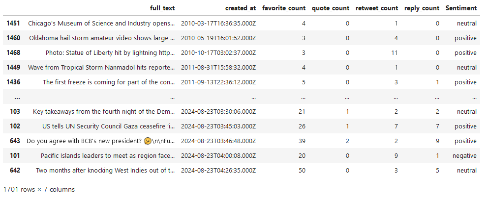
Now, this dataset is looking ready for classification, something which won’t take much time.

4. Sentiment analysis with machine learning

The text we've preprocessed is ready for sentiment analysis. Now comes the easier part of using this data to train our Machine Learning model. Every supervised ML model’s training involves some key steps.

• Splitting the dataset
• Encoding
• Choosing the suitable classification algorithm
• Optimization/training
• Evaluation

Split the dataset

The dataset will be split into training and testing segments. For that, we'll use Scikit-learn’s train_test_split. Setting a fixed random state ensures we can reproduce our results deterministically.

from sklearn.model_selection import train_test_split
randomState = 5

X_train, X_test, y_train, y_test = train_test_split(tweets_data['full_text'],tweets_data['sentiment'], test_size=0.2, random_state=randomState)

train_df = pd.DataFrame({'full_text': X_train, 'sentiment': y_train})
test_df = pd.DataFrame({'full_text': X_test, 'sentiment': y_test})

We'll also continue using data frames to split the dataset. In the next section, we'll see how helpful they are when we analyze the results.

Encoding

As you know, neural networks or any ML algorithm works on numerical data, so we need to convert the preprocessed data using some encoding algorithm. There are some encoders available, for example:

• Bag of words - in the simplest of methods, we make a lexicon and count the frequency of each word in that lexicon. We have encoders like Count Vectorizer or TF-IDF (both available in Scikit-learn) or TF-IDF Vectorizer available for the purpose.
• Word embeddings - pre-trained word embeddings like Word2Vec or GloVe are commonly used for vectorization.
• Tokenizers for transformer models - many transformer models, like BERT, Whisper, Phi, etc., come with their own pre-trained tokenizers. We can readily use them for encoding. I would recommend using HuggingFace’s AutoTokenizer here.

We'll use TF-IDF (Term Frequency-Inverse Document Frequency) to get representation using the frequency of terms.

from sklearn.feature_extraction.text import TfidfVectorizer, CountVectorizer

tfidf_vectorizer = TfidfVectorizer()

tfidf_features_train = tfidf_vectorizer.fit_transform(X_train)
tfidf_features_test = tfidf_vectorizer.transform(X_test)

"""
#You can uncomment this code if you want to use the count vectorizer features instead.
count_vectorizer = CountVectorizer()

cv_features_train = count_vectorizer.fit_transform(X_train)
cv_features_test = count_vectorizer.transform(X_test)
"""

You may have noticed that we use just transform() for the testing features but fit_transform() for the training ones. This function ensures that we first fit/train the data and then transform it.

Classification algorithms

While it's pretty common to use deep models, especially Transformers, for NLP (or even Vision) tasks, we shouldn't forget that other models/algorithms like LSTMs, RNNs, or even classical models like SVM or Naive Bayes can also be used for sentiment classification (or any other NLP task) - especially for smaller amount of data.

Here, I'll use Support Vector Machines as its easy to use, quite fast and performs well across a wide variety of tasks.

We can use SVM with either a linear or some non-linear kernel. Usually, the RBF one (which uses the Gaussian kernel) gives the best results, so we'll use it to fit both sets of features (TF-IDF and Count Vectorizer ones).

from sklearn.svm import SVC

svm_model = SVC(kernel='rbf', random_state=randomState)

Training and evaluation

Using this model, we'll train and then test this model.

from sklearn.metrics import accuracy_score

svm_model.fit(tfidf_features_train, y_train)

y_pred = svm_model.predict(tfidf_features_test)
accuracy = accuracy_score(y_test, y_pred)
#66.57%

66% is not a bad result by any means for this small dataset. But we need to realize a couple of facts:

• VADER’s accuracy is around 80%, which means that our model is trained with a fair amount of noise (which is lower than the human annotation).
• Annotating for sentiment analysis is not easy. There are a number of text samples where even human judgment can be on the borderline. For example, a tweet “Vehicle-to-Everything underpinned by 5G connectivity allows for the real-time delivery of enhanced driving information. See how #V2X and #5G are shaping the future of connected driving” is determined neutral by VADER, but positive by the SVM and none of them is wrong.

Note: In a real project, it would be preferable to obtain higher-quality labels through human annotation or even use LLM annotation, which would be a definite improvement over VADER. For example, I used Hugging Face’s roBERTa model to relabel the data, and it improved the accuracy beyond 70%.

Here's the code snippet you can use to replace VADER's sentiment labels with those generated by a transformer model:

from transformers import pipeline

sentiment_pipeline = pipeline("sentiment-analysis", model="cardiffnlp/twitter-roberta-base-sentiment", tokenizer=AutoTokenizer.from_pretrained("cardiffnlp/twitter-roberta-base-sentiment")) #Please feel free to use Model of your own choice

df = pd.read_csv("consolidatedTweets.csv")
df['label'] = df['full_text'].apply(lambda x: sentiment_pipeline(x)[0]['label'])

df[['full_text', 'label']].to_csv("consolidatedTweets_HFLabels.csv", index=False)

Interestingly, I tried it with CV features, and it came back with similar accuracy (65.10%), though a closer inspection shows different precision, recall, etc. This is itself a whole topic and readers are encouraged to explore more about it.

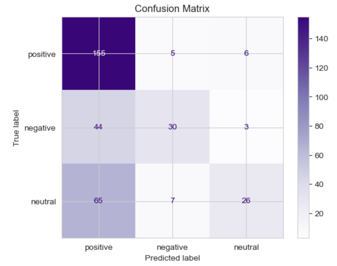
To summarize the results, here's the confusion matrix. As we can see, the model is a bit skewed towards the positive predictions, but the reason is evident here too: we have unbalanced data with a much higher representation of positive than neutral or negative samples.

5. Visualizing sentiment analysis results

Beyond these numbers, we can visualize these results in more meaningful ways too. Let’s round this up with some visual analyses.

Plotting sentiment scores

We used VADER to label the training dataset and can’t ignore its significance in our model. If we plot the histogram of its scores, it shows that lots of tweets have ‘neutral’ content, which is understandable.

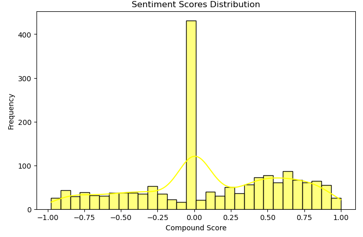
Here's the code for reference.

import matplotlib.pyplot as plt
import seaborn as sb

df['compound_sentiment_score'] = tweets_data['full_text'].apply(lambda text: analyzer.polarity_scores(text)['compound'])

plt.figure(figsize=(8, 5))
sb.histplot(df['compound_sentiment_score'], bins=30, kde=True, color='yellow')
plt.title('Sentiment Scores Distribution')
plt.xlabel('Compound Score')
plt.ylabel('Frequency')
plt.show()

An even more interesting way of visualizing these results will be word clouds.

Word clouds

WordCloud is a library that shows words graphically in terms of their relative frequency. And I'm sure these sorts of charts aren’t something you would be unaware of. We can install WordCloud as:

pip install wordcloud

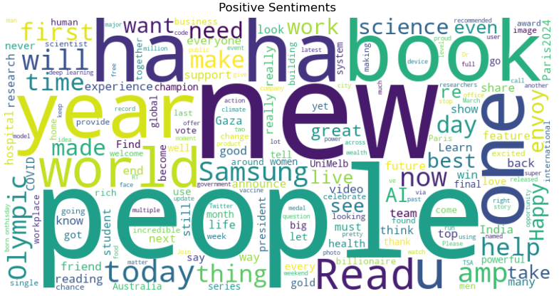
We can use the WordCloud class to instantiate the respective object (with parameters like height, width, etc.). Using it in conjunction with Matplotlib, we can show word clouds for all 3 sentiments.

from wordcloud import WordCloud
import matplotlib.pyplot as plt

excluded_words = {'https', 't', 'co', 'S'}
stopwords = set(WordCloud().stopwords)
stopwords.update(excluded_words)

text_for_sentiment = tweets_data[tweets_data['sentiment'] == 'positive']['full_text'].str.cat(sep=' ')
wordcloud = WordCloud(width=800, height=400, background_color='white', stopwords=stopwords).generate(text_for_sentiment)

plt.figure(figsize=(10, 5))
plt.imshow(wordcloud, interpolation='bilinear')
plt.axis('off')
plt.title('Positive Sentiments')
plt.show()

Using this code, we can see some useful connections between the words and sentiments.

Positive sentiments

Some of the terms like “Read, world, Olympic, people, book, Happy, make” are pretty implicit.

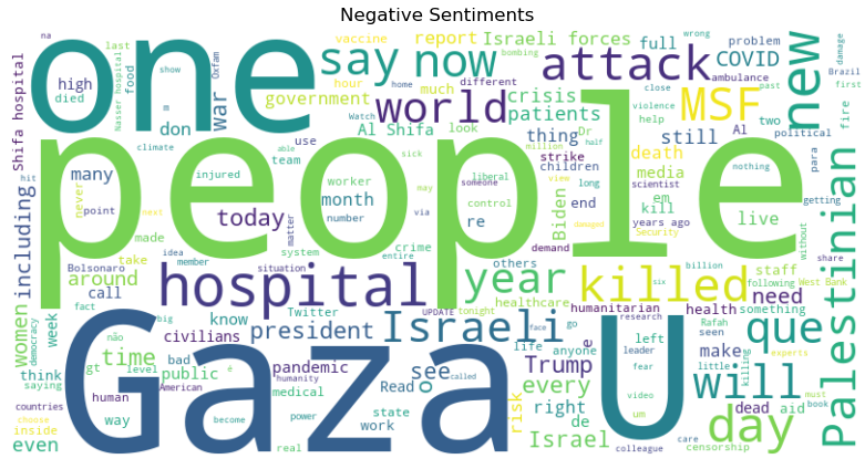
Negative sentiments

If we update the sentiment to negative in the code above, we get the desired word cloud. It's pretty obvious to see the tweets involving the mention of Gaza, a hospital, someone killed, Doctors without Borders (MSF), some attacks, or COVID (these tweets are from the 2010s so include some COVID-era data as well). Seeing “people” featuring in both positive and negative sentiments gives both concerns and hope about the future of humanity.

Neutral sentiments

Finally, there's a word cloud for those words that feature most in neutral sentiment tweets (if you remember, the histogram peaked at the center). I'm personally surprised to see “Taxes” featured there twice and without emotion.

Best practices for sentiment analysis

• Try to have a balanced dataset — usually news is a combination of both positive and negative sentiments. On the other hand, business accounts (expectedly) rarely post anything negative, so try to have a dataset with a good balance.
• Don’t over-preprocess — it depends on your specific requirements, but if in doubt, you can try using both types of data.
• Use hyperparameter tuning — to get optimum results for a given classifier. It’s much easier to perform for simpler classification algorithms but gets expensive with deeper models and more data.

Get data for sentiment analysis

Tap into a library of battle-tested scrapers from fellow developers

Get started on a free Apify plan — no setup required

Sign up now and start scraping

Summary

We started by installing the necessary libraries and then scraped and created our own datasets.

For preprocessing, we applied techniques that are not exclusive to sentiment analysis but useful across various NLP tasks.

VADER proved effective for both analyzing the sentiment of individual sentences and labeling entire unlabelled datasets.

The training process we used is adaptable to a wide range of NLP tasks and can be extended to other Machine Learning applications.

Finally, we demonstrated how WordCloud can visually represent sentiment distribution in a dataset.